구글에서 진행했던 조대협님의 텐소플로우 강의와 김성 교수님의 강의를 듣고 개인적으로 공부하면서 정리한 내용입니다
아래 소스는 김성 교수님 강의의 소스를 그대로 가져왔고, 수업을 들으면서 주석으로 정리한 부분입니다
Logistic Classification
두 개의 결과(true or false)를 구분할 때 사용하며, Logistic(=Sigmoid)를 이용하여 0 or 1로 값을 바꿔서 구분을 할 수 있게 해줍니다
Logistic Hypothesis
hypothesis = tf.sigmoid(tf.matmul(X, W) + b)
Logistic Cost Function
cost = -tf.reduce_mean(Y * tf.log(hypothesis) + (1 - Y) * tf.log(1-hypothesis))
optimizer = tf.train.GradientDescentOptimizer(learning_rate=0.01).minimize(cost)
실습 #1
소스
import tensorflow as tf

# Logistic(=Sigmoid)

x_data = [[1, 2], [2, 3], [3, 1], [4, 3], [5, 3], [6, 2]]
y_data = [[0], [0], [0], [1], [1], [1]]

X = tf.placeholder(tf.float32, shape=[None, 2]) # shape[n개, 들어오는 개수]
Y = tf.placeholder(tf.float32, shape=[None, 1]) # shape[n개, 나가는 개수]

# tf.random_normal() 정규분포로부터의 난수값을 반환
W = tf.Variable(tf.random_normal([2, 1]), name='weight') # random_normal([X의 개수, Y의 개수]) = random_normal([들어오는 개수, 나가는 개수])
b = tf.Variable(tf.random_normal([1], name='bias')) # random_normal([Y의 개수]) = random_normal([나가는 개수])

hypothesis = tf.sigmoid(tf.matmul(X, W) + b)

# Cost/Loss Function, 모델에 맞춰서 이부분만 외워주면 됨
cost = -tf.reduce_mean(Y * tf.log(hypothesis) + (1 - Y) * tf.log(1 - hypothesis))

# Optimize
optimizer = tf.train.GradientDescentOptimizer(learning_rate=0.01).minimize(cost)

predicted = tf.cast(hypothesis > 0.5, dtype=tf.float32) # tf.cast() : dtype으로 바꿔줌, 0.5이상이면 1(=true), 아니면 0(=false)
accuracy = tf.reduce_mean(tf.cast(tf.equal(predicted, Y), dtype=tf.float32)) # tf.cast -> True = 1, False = 0

with tf.Session() as sess:
  sess.run(tf.global_variables_initializer())

  for step in range(10001):
    cost_val, _ = sess.run([cost, optimizer], feed_dict={X: x_data, Y:y_data})

    if step % 200 == 0:
      print(step, cost_val)

  h, c, a  = sess.run([hypothesis, predicted, accuracy], feed_dict={X: x_data, Y: y_data})
  print("\nHypothesis: ", h, "\nCorrect (Y): ", c, "\nAccuracy: ", a)
결과
(0, 3.8896148)
(200, 0.83243585)
(400, 0.6960969)
(600, 0.62942082)
(800, 0.58893687)
(1000, 0.55947894)
(1200, 0.53534669)
(1400, 0.51416087)
(1600, 0.49483705)
(1800, 0.47684574)
(2000, 0.45991191)
(2200, 0.44388333)
(2400, 0.42866847)
(2600, 0.41420662)
(2800, 0.40045273)
(3000, 0.38736966)
(3200, 0.37492433)
(3400, 0.36308578)
(3600, 0.35182416)
(3800, 0.34111068)
(4000, 0.33091721)
(4200, 0.32121679)
(4400, 0.31198281)
(4600, 0.30319014)
(4800, 0.29481432)
(5000, 0.28683224)
(5200, 0.2792218)
(5400, 0.27196193)
(5600, 0.26503286)
(5800, 0.25841579)
(6000, 0.25209311)
(6200, 0.24604814)
(6400, 0.24026521)
(6600, 0.23472951)
(6800, 0.22942738)
(7000, 0.22434586)
(7200, 0.21947266)
(7400, 0.2147965)
(7600, 0.21030669)
(7800, 0.20599319)
(8000, 0.20184655)
(8200, 0.19785808)
(8400, 0.19401939)
(8600, 0.19032289)
(8800, 0.18676127)
(9000, 0.18332762)
(9200, 0.18001568)
(9400, 0.17681932)
(9600, 0.17373295)
(9800, 0.17075126)
(10000, 0.16786921)
('\nHypothesis: ', array([[ 0.0388297 ],
       [ 0.16854469],
       [ 0.34149736],
       [ 0.76511103],
       [ 0.92886275],
       [ 0.9766435 ]], dtype=float32), '\nCorrect (Y): ', array([[ 0.],
       [ 0.],
       [ 0.],
       [ 1.],
       [ 1.],
       [ 1.]], dtype=float32), '\nAccuracy: ', 1.0)
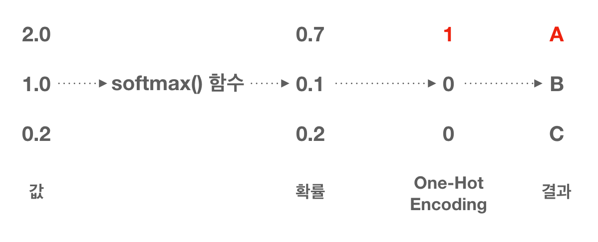
Softmax Classification
여러개의 결과를 구분할 때 사용
Softmax Hypothesis
# X : 입력값 / Y : 결과값 (내가 가지고 있는 데이터)
# W : Weight / b : bias (hypothesis를 통해 두 변수의 최적의 값을 찾는게 목적)

logits = tf.matmul(X, W) + b
hypothesis = tf.nn.softmax(logits)
Softmax Cost Function
# X : 입력값 / Y : 결과값 (내가 가지고 있는 데이터)
# W : Weight / b : bias (hypothesis를 통해 두 변수의 최적의 값을 찾는게 목적)

cost = tf.reduce_mean(-tf.reduce_sum(Y*tf.log(hypothesis), axis=1))
optimizer = tf.train.GradientDescentOptimizer(learning_rate=0.1).minimize(cost)
One Hot Encoding
여러개의 결과가 있을때 결과에 가장 근사값만 1로 나머지는 0으로 표시함으로써 구분할 수 있게 해준다.
실습 #1
import tensorflow as tf

x_data = [[1, 2, 1, 1], [2, 1, 3, 2], [3, 1, 3, 4], [4, 1, 5, 5], [1, 7, 5, 5], [1, 2, 5, 6], [1, 6, 6, 6], [1, 7, 7, 7]]
y_data = [[0, 0, 1], [0, 0, 1], [0, 0, 1], [0, 1, 0], [0, 1, 0], [0, 1, 0], [1, 0, 0], [1, 0, 0]]

X = tf.placeholder(tf.float32, [None, 4]) # 위의 x_data가 4개라서
Y = tf.placeholder(tf.float32, [None, 3]) # 위의 y_data가 3개라서
nb_classes = 3

W = tf.Variable(tf.random_normal([4, nb_classes]), name='weight') # Weight는 [입력값, 출력값]을 차원으로 가진다
b = tf.Variable(tf.random_normal([nb_classes]), name='bias') # bias는 y의 출력값을 차원으로 가진다

# hypothesis
hypothesis = tf.nn.softmax(tf.matmul(X, W) + b)

cost = tf.reduce_mean(-tf.reduce_sum(Y*tf.log(hypothesis), axis=1)) # axis = 축
optimizer = tf.train.GradientDescentOptimizer(learning_rate=0.1).minimize(cost)

# Training
with tf.Session() as sess:
  sess.run(tf.global_variables_initializer())

  for step in range(2001):
    sess.run(optimizer, feed_dict={X: x_data, Y: y_data})

    if step % 200 == 0:
      print(step, sess.run(cost, feed_dict={X: x_data, Y: y_data}))


  # Test
  ## 입력이 1개일때 : 위에서 트레이닝을 통해 생성된 hypothesis에 [1, 11, 7, 9]를 대입했을때 어떻게 나오는지
  a = sess.run(hypothesis, feed_dict={X:[[1, 11, 7, 9]]})
  print(a, sess.run(tf.arg_max(a,1))) # tf.arg_max는 가장 큰 값을 골라서 주는것

  ## 입력이 1개일때 : 위에서 트레이닝을 통해 생성된 hypothesis에 [1, 11, 7, 9]를 대입했을때 어떻게 나오는지
  all = sess.run(hypothesis, feed_dict={X: [ [1, 11, 7, 9],
                                             [1, 3, 4, 3],
                                             [1, 1, 0, 1]]})
  print (all, sess.run(tf.arg_max(all,1)))
결과
(0, 1.2109271)
(200, 0.46954274)
(400, 0.37738693)
(600, 0.29948664)
(800, 0.24126217)
(1000, 0.21734878)
(1200, 0.19782056)
(1400, 0.18149593)
(1600, 0.16762473)
(1800, 0.1556862)
(2000, 0.14530227)
(array([[  2.13616993e-03,   9.97854173e-01,   9.59866247e-06]], dtype=float32), array([1]))
(array([[  2.13616993e-03,   9.97854173e-01,   9.59866247e-06],
       [  9.02791023e-01,   8.50417688e-02,   1.21671809e-02],
       [  6.99110547e-09,   2.95337552e-04,   9.99704659e-01]], dtype=float32), array([1, 0, 2]))
실습 #2 (당뇨병 예측하기)
소스 받기
!curl https://raw.githubusercontent.com/hunkim/DeepLearningZeroToAll/master/data-03-diabetes.csv > data-03-diabetes.csv
소스
import tensorflow as tf
import numpy as np

xy = np.loadtxt('data-03-diabetes.csv', delimiter=',', dtype=np.float32) # 8개가 피처, 마지막 1개가 결과(1=당뇨병 / 0=!당뇨병)
x_data = xy[:, 0:-1]
y_data = xy[:, [-1]]

X = tf.placeholder(tf.float32, shape=[None, 8]) # X의 데이터가 8개, Feature개수
Y = tf.placeholder(tf.float32, shape=[None, 1]) # Y의 데이터는 1개

W = tf.Variable(tf.random_normal([8, 1]), name='weight')
b = tf.Variable(tf.random_normal([1]), name='bias')

hypothesis = tf.sigmoid(tf.matmul(X, W) + b)

cost = -tf.reduce_mean(Y * tf.log(hypothesis) + (1 - Y) * tf.log(1 - hypothesis))
train = tf.train.GradientDescentOptimizer(learning_rate=0.01).minimize(cost)

predicted = tf.cast(hypothesis > 0.5, dtype=tf.float32)
accuracy = tf.reduce_mean(tf.cast(tf.equal(predicted, Y), dtype=tf.float32))

with tf.Session() as sess:
  sess.run(tf.global_variables_initializer())

  feed = {X: x_data, Y: y_data}
  for step in range(10001):
    sess.run(train, feed_dict=feed)

    if step % 2000 == 0:
      print(step, sess.run(cost, feed_dict=feed))

  h, c, a = sess.run([hypothesis, predicted, accuracy], feed_dict=feed)
  print("\nHypothesis: ", h, "\nCorrect (Y): ", c, "\nAccuracy: ", a)
결과
(0, 0.95397258)
(2000, 0.63290697)
(4000, 0.54697829)
(6000, 0.51436806)
(8000, 0.49879706)
(10000, 0.49010789)
('\nHypothesis: ', array([[ 0.3804661 ],
       [ 0.89527673],
       [ 0.33242166],
       [ 0.94499367],
       [ 0.20146242],
       [ 0.78935677],
       [ 0.95599049],
       [ 0.66131264],
       [ 0.2867631 ],
       [ 0.50592452],
       ...
       [ 1.],
       [ 0.],
       [ 1.],
       [ 0.],
       [ 1.],
       [ 1.],
       [ 1.],
       [ 1.],
       [ 1.],
       [ 1.]], dtype=float32), '\nAccuracy: ', 0.770751)
softmax_cross_entropy_with_logits() 함수
아래에서 Softmax Cost 함수를 만드는 2개의 방법을 설명하는데 같은건데, #2는 softmax_cross_entropy_with_logits()를 사용
Softmax Cost 함수 만들기 #1
logits = tf.matmul(X, W) + b # score라고도 부름
hypothesis = tf.nn.softmax(logits)
cost = tf.reduce_mean(-tf.reduce_sum(Y * tf.log(hypothesis), axis=1))
Softmax Cost 함수 만들기 #2
logits = tf.matmul(X, W) + b # score라고도 부름
cost_i = tf.nn.softmax_cross_entropy_with_logits(logits=logits, labels=Y_one_hot)
cost = tf.reduce_mean(cost_i)
실습 #2
우선 실습 데이터 받기
!curl https://raw.githubusercontent.com/hunkim/DeepLearningZeroToAll/master/data-04-zoo.csv > data-04-zoo.csv
실습 소스
import tensorflow as tf
import numpy as np

xy = np.loadtxt('data-04-zoo.csv', delimiter=',', dtype=np.float32)
x_data = xy[:, 0:-1] # 0~n-1
y_data = xy[:, [-1]] # n

nb_classes = 7 # 0~6개의 숫자라 7개

X = tf.placeholder(tf.float32, [None, 16])

# 중요 One Hot이 아닌 값을 One Hot으로 reshape 하기
Y = tf.placeholder(tf.int32, [None, 1]) # 0 ~ 6의 숫자를 하나에 담아 주기 위함 shape=(n, 1)
Y_one_hot = tf.one_hot(Y, nb_classes) # one_hot()를 쓰면 한 차원이 증가하게 된다 shape=(n, 1, 7)
Y_one_hot = tf.reshape(Y_one_hot, [-1, nb_classes]) # 위에서 한 차원이 증가해서 다시 reshape 함 shape=(n, 7)

W = tf.Variable(tf.random_normal([16, nb_classes]), name='weight')
b = tf.Variable(tf.random_normal([nb_classes]), name='bias')

logits = tf.matmul(X, W) + b
hypothesis = tf.nn.softmax(logits)

cost_i = tf.nn.softmax_cross_entropy_with_logits(logits=logits, labels=Y_one_hot)

cost = tf.reduce_mean(cost_i)
optimizer = tf.train.GradientDescentOptimizer(learning_rate=0.1).minimize(cost)

prediction = tf.argmax(hypothesis, 1) # Probability 0 ~ 6중 1나를 만들겠다는 의미
correct_prediction = tf.equal(prediction, tf.argmax(Y_one_hot, 1))
accuracy = tf.reduce_mean(tf.cast(correct_prediction, tf.float32)) # tf.cast() : Tensor를 dtype으로 변환

with tf.Session() as sess:
  sess.run(tf.global_variables_initializer())

  for step in range(2000):
    sess.run(optimizer, feed_dict={X: x_data, Y: y_data})

    if step % 100 == 0:
      loss, acc = sess.run([cost, accuracy], feed_dict={X: x_data, Y: y_data})
      print("Step: {:5}\tLoss: {:.3f}\tAcc: {:.2%}".format(step, loss, acc))

  pred = sess.run(prediction, feed_dict={X: x_data})

  for p, y, in zip(pred, y_data.flatten()): # flatten : [[1], [0]] -> [1, 0]
                  print("[{}] Prediction: {} True Y: {}".format(p == int(y), p, int(y)))
결과
Step:     0	Loss: 4.289	Acc: 15.84%
Step:   100	Loss: 0.748	Acc: 79.21%
Step:   200	Loss: 0.451	Acc: 89.11%
Step:   300	Loss: 0.336	Acc: 91.09%
Step:   400	Loss: 0.268	Acc: 93.07%
Step:   500	Loss: 0.222	Acc: 93.07%
Step:   600	Loss: 0.189	Acc: 94.06%
Step:   700	Loss: 0.164	Acc: 96.04%
Step:   800	Loss: 0.144	Acc: 96.04%
Step:   900	Loss: 0.129	Acc: 97.03%
Step:  1000	Loss: 0.116	Acc: 98.02%
Step:  1100	Loss: 0.105	Acc: 98.02%
Step:  1200	Loss: 0.097	Acc: 99.01%
Step:  1300	Loss: 0.089	Acc: 100.00%
Step:  1400	Loss: 0.083	Acc: 100.00%
Step:  1500	Loss: 0.077	Acc: 100.00%
Step:  1600	Loss: 0.072	Acc: 100.00%
Step:  1700	Loss: 0.068	Acc: 100.00%
Step:  1800	Loss: 0.064	Acc: 100.00%
Step:  1900	Loss: 0.060	Acc: 100.00%
[True] Prediction: 0 True Y: 0
[True] Prediction: 0 True Y: 0
[True] Prediction: 3 True Y: 3
[True] Prediction: 0 True Y: 0
[True] Prediction: 0 True Y: 0
[True] Prediction: 0 True Y: 0
[True] Prediction: 0 True Y: 0
[True] Prediction: 3 True Y: 3
[True] Prediction: 3 True Y: 3
[True] Prediction: 0 True Y: 0
[True] Prediction: 0 True Y: 0
[True] Prediction: 1 True Y: 1
[True] Prediction: 3 True Y: 3
[True] Prediction: 6 True Y: 6
[True] Prediction: 6 True Y: 6
[True] Prediction: 6 True Y: 6
[True] Prediction: 1 True Y: 1
[True] Prediction: 0 True Y: 0
[True] Prediction: 3 True Y: 3
[True] Prediction: 0 True Y: 0
[True] Prediction: 1 True Y: 1
[True] Prediction: 1 True Y: 1
[True] Prediction: 0 True Y: 0
[True] Prediction: 1 True Y: 1
[True] Prediction: 5 True Y: 5
[True] Prediction: 4 True Y: 4
[True] Prediction: 4 True Y: 4
[True] Prediction: 0 True Y: 0
[True] Prediction: 0 True Y: 0
[True] Prediction: 0 True Y: 0
[True] Prediction: 5 True Y: 5
[True] Prediction: 0 True Y: 0
[True] Prediction: 0 True Y: 0
[True] Prediction: 1 True Y: 1
[True] Prediction: 3 True Y: 3
[True] Prediction: 0 True Y: 0
[True] Prediction: 0 True Y: 0
[True] Prediction: 1 True Y: 1
[True] Prediction: 3 True Y: 3
[True] Prediction: 5 True Y: 5
[True] Prediction: 5 True Y: 5
[True] Prediction: 1 True Y: 1
[True] Prediction: 5 True Y: 5
[True] Prediction: 1 True Y: 1
[True] Prediction: 0 True Y: 0
[True] Prediction: 0 True Y: 0
[True] Prediction: 6 True Y: 6
[True] Prediction: 0 True Y: 0
[True] Prediction: 0 True Y: 0
[True] Prediction: 0 True Y: 0
[True] Prediction: 0 True Y: 0
[True] Prediction: 5 True Y: 5
[True] Prediction: 4 True Y: 4
[True] Prediction: 6 True Y: 6
[True] Prediction: 0 True Y: 0
[True] Prediction: 0 True Y: 0
[True] Prediction: 1 True Y: 1
[True] Prediction: 1 True Y: 1
[True] Prediction: 1 True Y: 1
[True] Prediction: 1 True Y: 1
[True] Prediction: 3 True Y: 3
[True] Prediction: 3 True Y: 3
[True] Prediction: 2 True Y: 2
[True] Prediction: 0 True Y: 0
[True] Prediction: 0 True Y: 0
[True] Prediction: 0 True Y: 0
[True] Prediction: 0 True Y: 0
[True] Prediction: 0 True Y: 0
[True] Prediction: 0 True Y: 0
[True] Prediction: 0 True Y: 0
[True] Prediction: 0 True Y: 0
[True] Prediction: 1 True Y: 1
[True] Prediction: 6 True Y: 6
[True] Prediction: 3 True Y: 3
[True] Prediction: 0 True Y: 0
[True] Prediction: 0 True Y: 0
[True] Prediction: 2 True Y: 2
[True] Prediction: 6 True Y: 6
[True] Prediction: 1 True Y: 1
[True] Prediction: 1 True Y: 1
[True] Prediction: 2 True Y: 2
[True] Prediction: 6 True Y: 6
[True] Prediction: 3 True Y: 3
[True] Prediction: 1 True Y: 1
[True] Prediction: 0 True Y: 0
[True] Prediction: 6 True Y: 6
[True] Prediction: 3 True Y: 3
[True] Prediction: 1 True Y: 1
[True] Prediction: 5 True Y: 5
[True] Prediction: 4 True Y: 4
[True] Prediction: 2 True Y: 2
[True] Prediction: 2 True Y: 2
[True] Prediction: 3 True Y: 3
[True] Prediction: 0 True Y: 0
[True] Prediction: 0 True Y: 0
[True] Prediction: 1 True Y: 1
[True] Prediction: 0 True Y: 0
[True] Prediction: 5 True Y: 5
[True] Prediction: 0 True Y: 0
[True] Prediction: 6 True Y: 6
[True] Prediction: 1 True Y: 1